
AP Stats Exam Prep Meets Data Careers
- Admin
- Apr 3, 2024
- 6 min read

Updated: Apr 17, 2024
Need some practice problems for your AP Stats students to help them prepare for the AP Exam? Want them to learn a little bit more about potential career paths in statistics and data science along the way? We have you covered with these practice problems! Sparse solutions can be found at the bottom of the post, but stay tuned to the section's social media account for detailed threads each weekday April 8th-19th featuring a step-by-step solution, plus some career information related to each problem.
2 sample proportion
James is interested in whether projects on OSF (an open science platform) with open data (data that is available for download) are more replicable than projects without open data. He collects separate random samples of projects from OSF. Here are the results:
Replicates? | Open Data | No Open Data |
Yes | 75 | 64 |
No | 25 | 136 |
Total | 100 | 200 |
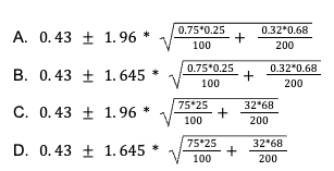
James wants to use these results to construct a 95% confidence interval to estimate the difference in the proportion of projects that reproduce (open - not). Assuming all the necessary conditions for inference are met, which of the following is the correct confidence interval for James’s question?
Chi-squared
Jason is interested in whether your favorite programming language (R vs. Python) is independent of your job title (Statistician vs. Data Engineer). Write out the null and alternative hypothesis for this Chi-Square Test of Independence, and then calculate the Chi-square test statistic and p-value. Note: accompanying R code can be found here.
Statistician | Data Engineer | Total | |
R | 76 | 33 | 109 |
Python | 24 | 67 | 91 |
Total | 100 | 100 | 200 |
Difference in means
A random sample of 50 American Statistical Association (ASA) members who work in a federal government job whose terminal degree is a Masters degree were asked about their salary. Similarly, a random sample of 50 American Statistical Association members who work in a federal government job whose terminal degree is a PhD were asked about their salary. The mean in the Masters degree group is 119.92 (in thousands of dollars) with a standard deviation of 18.4. The mean in the PhD group is 152.21 (in thousands of dollars) with a standard deviation of 24.52.
Is there evidence at the 99% level that the average salary for an ASA member who works in a federal government job with a terminal Master’s degree is less than that of an ASA member who works in a federal government job with a terminal PhD?
*Note: The summary statistics here are informed by page 13 of this survey. Accompanying R code can be found here.
Regression
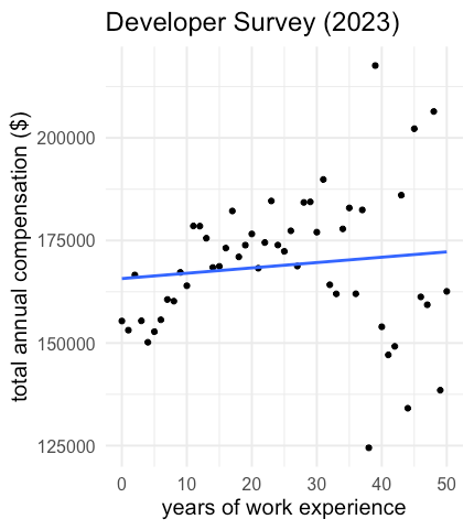
In 2023, a popular website for data enthusiasts asked computer developers to respond to their annual survey. Two questions on the survey include what their yearly compensation is and how many years of experience they have. Here is a plot of the data along with the line of best fit.
a.) What type of sample do you think would result from data collected in this way. Explain your reasoning.
b.) Describe the shape, direction, and strength of the relationship you see in the above figure.
c.) Which of the following lines of best fit is representative of this data? Explain your reasoning.
Compensation = 165708.1 + 130.2 * WorkExp
Compensation = 165708.1 - 130.2 * WorkExp
d.) Interpret the slope for the line of best fit you chose.
e.) Interpret the y-intercept of the line of best fit you chose.
f.) Predict the salary for a developer with 3 years of experience.
g.) Suppose a developer with 3 years of experience reported a salary of $150,000 What is the residual for this observation?
Note: The data here are informed by this survey. Accompanying R code can be found here.
Experimental design
Jenna is interested in whether taking an improv class improves the readability of scientists’ papers. She takes a group of scientists and splits them into 4 groups: Engineering and Math, Literature and History, Biology and Chemistry, and Business. Within each of these groups, Jenna randomly assigns half the faculty to attend an improv class once a week for 3 months, and half to attend a fiction book club. Then, she uses an established measure of readability to rate the readability of the faculty members’ papers published within 6 months. Which of the following best describes the design of the study?
A. Completely randomized
B. Randomized block
C. Matched-pairs design
D. Double-blind
Geometric distribution
Andy estimates that he gets initial interviews from 12% of jobs he applies to. Find the probability that Andy will have to apply to 10 jobs before getting his first interview. Round your answer to the nearest hundredth.
Combinatorics
Jasper works at a startup called VentureAI. His team consists of a Data Scientist, Data Analyst, Data Engineer, Statistician, and Machine Learning Engineer.
How many different sub-teams of 3 (order does not matter) can Jasper’s VentureAI team form?
Percentile/Z-score
*Note: The summary statistics here are informed by Table 6 of this report.
a.) Female academic faculty in mathematical sciences departments at the full professor level have a mean salary of $89,186. If the 90% percentile of this distribution is $206,000, what is the standard deviation of the distribution. You may assume that the distribution of salaries is roughly normal.
b.) Based on the standard deviation you calculated in the previous step, determine how many standard deviations away from the mean full professor Sally is with a salary of $95,000. If you got stuck on part a.) pick a standard deviation to use for this problem.
Comparing histograms
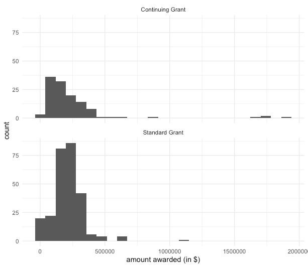
Compare the distributions of National Science Foundation (NSF) funding for statistics-related projects between standard grants and continuing grants. Remember to discuss center, spread, shape, and potential outliers.
Confidence intervals
A random sample of 100 data analysts at a company were asked how many hours a week they spend talking on the phone or on video calls with a collaborator or stakeholder at two points during their career. This was done in 2019 (before the start of the COVID-19 pandemic) and in 2021 (after the start of the COVID-19 pandemic). In 2019, the mean of the reported hours was 6.84 with a standard deviation of 1.79. In 2021, the mean of the reported hours was 14.28 with a standard deviation of 1.64.

a.) Compute and interpret in context a 95% confidence interval for the mean difference in hours spent talking on the phone or on video calls with a collaborator or stakeholder. Be sure to check the conditions for inference before proceeding.
b.) Is there sufficient evidence to indicate a mean difference between the two years? Justify your conclusion.
Solutions
Remember to stay tuned to the section's social media account for detailed threads each weekday April 8th-19th featuring a step-by-step solution, plus some career information related to each problem.
2 sample proportion:
A
Chi-squared:
Null Hypothesis: Favorite programming language and job title are independent. There is no association between them.
Alternative Hypothesis: Favorite programming language and job title are not independent. There is an association between them.
Test statistic: 35.57
p-value: 2.4 e-09 (really small)
Difference in means:
Check Conditions
First, we note that we have two independent samples. We don’t think that the Masters degree group has any natural pairing with the PhD group. We have random samples from both populations. We do not know if the populations are normally distributed, but we have large sample sizes, so we can lean on the Central Limit Theorem to ensure that that the distribution of the difference in means is approximately normal.
Hypotheses and Calculations
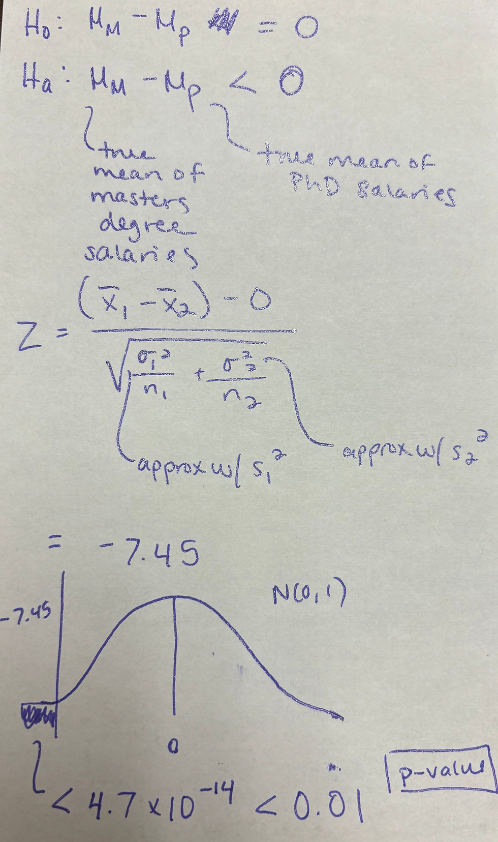
Interpret in Context
We reject the null hypothesis in favor of the alternative hypothesis. We have evidence in favor of the conclusion that the average salary for an ASA member who works in a federal government job with a terminal Master’s degree is less than that of an ASA member who works in a federal government job with a terminal PhD.
Regression:
a.) Volunteer sample - visitors to the website need to opt-in to the survey.
b.) Non-linear, positive, moderate relationship
c.) The first equation has a positive slope. Since we saw a positive relationship in the scatterplot, this is the appropriate line of best fit.
d.) For every extra year of experience, the total annual compensation for developers in 2023 increases on average by $130.20.
e.) The predicted starting salary of someone just starting a developer job in 2023 is $165,709.10.
f.) 165708.1 + 130.2 * 3 = $166,098.70
g.) observed - predicted = 150,000 - 166,098.70 = -$16,098.70
Experimental Design:
B
Geometric distribution:
0.03
Combinatorics:
10
Percentile/Z-score:

Comparing histograms:
Both distributions are right skewed. Most of the award values are less than $500,000 in both groups, but there are a few grants that awarded more than a million dollars. There seem to be more big awards (potential outliers) in the continuing grant group than the standard grant group.
Confidence intervals:
a.)
Check Conditions
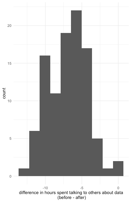
First, we note that we have two dependent samples; this is a before-and-after study on the same group of data analysts. We have a random sample of data analysts at a company. We do not know if the population is normally distributed, but we have a plot of the sample differences. The distribution is fairly symmetric and bell-shaped without any obvious outliers, so we will proceed.
Calculations
Note: a version of this blog post showed the wrong degrees of freedom. The rest of this solution was updated on 4/17/24 to fix that issue. Apologies!
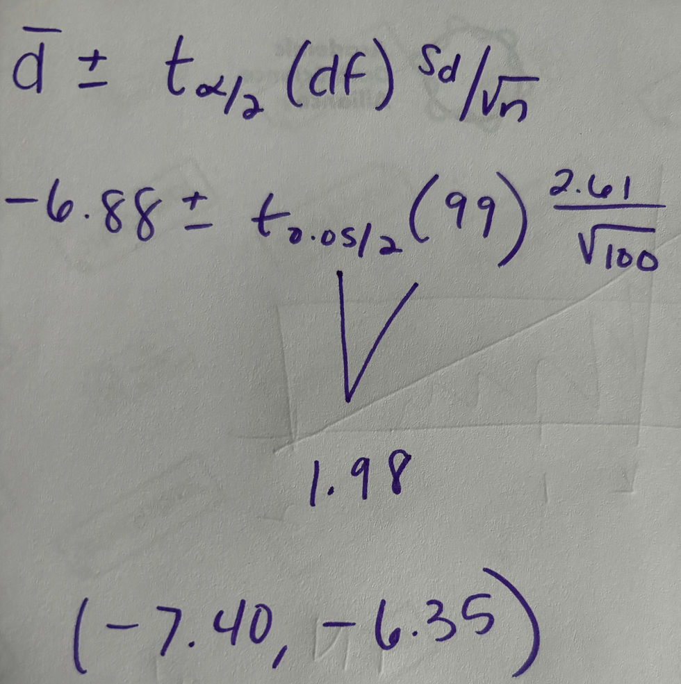
Interpret in Context
We are 95% confident that the true mean difference in hours spent talking to others about data is between -7.4 hours and -6.35 hours.
b.) Is there sufficient evidence to indicate a mean difference between the two years? Justify your conclusion.
Yes, the confidence interval does not contain 0, so we have evidence that there is a mean difference. In other words, no mean difference is not plausible.

Comments